mapmuts_enrichmentcorrelate.py

This is an analysis script for the output produced by mapmuts_inferenrichment.py. This script requires matplotlib to make the plots. It will raise an error if matplotlib is not available. This script also requires scipy in order to calculate correlation coefficients. However, you can still use the script if scipy is unavailable – you just won’t get any correlation coefficients.

The script takes as input the enrichment ratios in the enrichmentratios file(s) produced by mapmuts_inferenrichment.py and generates some useful correlation plots. All plots are on logarithmic scales since the enrichment scores are themselves ratios which naturally correspond to log scales.

The enrichmentratios files created by mapmuts_inferenrichment.py contain the following data for each mutation:

• The posterior mean enrichment ratio phi, along with the upper and lower limits of its 95% highest posterior density. This will always be a number > 0.
• The directratio, which is the enrichment calculate directly by dividing the counts in the selected by unselected libraries after subtracting errors. This number will typically be > 0, but it can also be zero, negative, or plus or minus infinity when the counts are very low (such that the estimated errors match or exceed the counts).
• The number of counts, mutdnacounts for the mutation in the input mutant library, which is roughly the denominator (before subtracting errors) for the enrichment ratio. This will be an integer >= 0. It gives some idea of how many counts went into determining phi and directratio – larger numbers of counts will typically correspond to more robust estimates.

Typically you would use this script for one of the following goals:

1. For a single library, you might want to compare how well phi the inferred enrichment ratio matches the direct directratio estimates. This program allows you to do this by generating a plot and calculating a Pearson correlation coefficient. You can also restrict your analysis to just include sites where mutdnacounts exceeds some cutoff (these are the sites with more data points).
2. For two (or more) libraries, you might want to compare the inferred enrichment ratios phi and the directratios between pairs of libraries. This script allows you to do this by generating plots and calculating correlation coefficients.

Running the script

To run this script, simply create an input file with the format described below. If you name your input file enrichmentcorrelate_infile.txt, then run the command:

mapmuts_enrichmentcorrelate.py enrichmentcorrelate_infile.txt

Input file

The input file is a text file with a series of key / value pairs. The required keys are indicated below. The values should not include spaces.

Lines beginning with # and empty lines are ignored.

Keys for the input file:

• enrichmentratios : A listing of the enrichment ratio files generated as *_enrichmentratios.txt by mapmuts_inferenrichment.py. You must list at least one file here, but can list more than one if you also want to look at correlations between pairs of samples. The files must exist, and the filenames cannot contain any spaces. To list multiple files, just separate them by spaces.
• samplenames : A listing of the sample names for each of the files specified by enrichmentratios. These are the names that are given to the samples in plots that compare across multiple samples. You must specify the same number of sample names here as you specify files under enrichmentratios, so there is one name for each corresponding sample. The sample names can NOT contain spaces, and different sample names are separated by spaces. However, if you include an underscore in the sample name then it is converted to a space in the actual plots.
• mutdnacounts_cutoff : One or more integers >= 0. Specifies the correlation plots should include only mutations for which mutdnacounts is >= the number specified here. Setting mutdnacounts_cutoff to zero means that all mutations will appear on the correlation plots. If you specify multiple numbers, then plots are created for each cutoff.
• plotdir specifies the directory where we place the plots. If you want them to be in the current directory, just make this ./. Otherwise specify some other directory, such as enrichmentcorrelations/. Directories specified by this prefix must already exist – nonexistent directories are NOT created, and an error will be raised if you specify a directory that does not already exist.
• limitadjustment specifies how we handle directratio values that are <= 0 or equal to inf (infinity). Because our plots are on a log scale, they can only handle finite ratios that are > 0. The enrichment values phi should satisfy this, but directratio will not always do so (for example if the numerator or denominator in the ratio is zero). In order to plot these values and calculate correlations, any values <= 0 are set to be equal to the minimum directratio that is > 0 divided by limitadjustment. Similarly, any value of directratio equal to inf is set to be equal to the maximum finite value of directratio times limitadjustment. For this to work, limitadjustment itself must be a number >= 1. If you set limitadjustment to one, then out of bounds values will be set to the maximum or minimum of the in-bounds values. This is somewhat sensible, but it may be preferable to set limitadjustment to a value such as 2 or 10 so that the out-of-bounds values are noticeably separated from those with actual plottable values of directratio.

Example input file

Here is an example input file:

# Input file for mapmuts_enrichmentcorrelate.py
enrichmentratios WT-1/WT-1_enrichmentratios.txt WT-2/WT-2_enrichmentratios.txt N334H-1/N334H-1_enrichmentratios.txt N334H-2/N334H-2_enrichmentratios.txt
samplenames WT-1 WT-2 N334H-1 N334H-2
mutdnacounts_cutoff 0 100
plotdir enrichmentcorrelations/
limitadjustment 2

Output

This script will write some brief output to standard out (sys.stdout) describing its progress.

IMPORTANT NOTE: The Pearson correlation coefficients are computed on the data as it is plotted. So these are correlations for the log-transformed data with any out-of-bounds points adjusted to in-range points as specified by limitadjustment.

Two types of plots are generated: plots comparing the inferred enrichment ratios phi with the direct estimates directratio, and plots comparing both phi and directratio across multiple samples (if more than one sample is specified). Both types of plots are in PDF format generated with matplotlib, and they include Pearson correlation coefficients if scipy is available. Specifically:

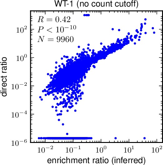
• For each sample and each mutdnacounts_cutoff, a plot of phi versus directratio is made. These plots only include mutations with values of mutdnacounts that are >= mutdnacounts_cutoff. The plots are named as */*_inferred_vs_direct_cutoff*.pdf where the first * is filled by plotdir, the second * by the sample name, and the third by the value of mutdna_cutoff. For example, for the input file above, a plot would be enrichmentcorrelations/WT-11_inferred_vs_direct_cutoff0.pdf. Here is an example of such a plot:

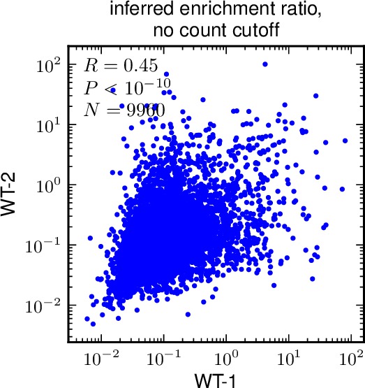
• If multiple samples are specified by enrichmentratios and samplenames, then plots are created that correlate the inferred enrichment ratios phi and the direct ratios directratio between all pairs of plots, making a separate plot for each cutoff specified by mutdnacounts_cutoff. The correlation plots include only those mutations for which both samples have values specified, and for which both samples have a number of counts that satisfies mutdnacounts_cutoff. The plots are named as */*_vs_*_inferred_cutoff*.pdf and */*_vs_*_direct_cutoff*.pdf where the first * is filled by plotdir, the second * by the first sample in a pair, the third * by the second sample in a pair, and the last * by the value of mutdna_cutoff. So for the above example input file, the names would be enrichmentcorrelations/WT-1_vs_WT-2_inferred_cutoff0.pdf, etc. Here is an example of such a plot: