mapmuts_preferencescorrelate.py

This is an analysis script for examining the correlations between amino-acid preferences \(\pi_{r,a}\) or differential preferences \(\Delta\pi_{r,a}\) from different analyses or samples.

It is designed to parse either the *_equilibriumpreferences.txt files created by mapmuts_inferpreferences.py or the differentialpreferences_selection_*.txt files created by mapmuts_inferdifferentialpreferences.py. It makes plots of the correlation between the amino-acid preferences or differntial preferences for all amino acids a at all sites r for multiple analyses or samples.

Dependencies

This script requires matplotlib to make the plots. It will raise an error if matplotlib is not available. This script also requires scipy in order to calculate correlation coefficients. However, you can still use the script if scipy is unavailable – you just won’t get any correlation coefficients.

Running the script

To run this script, simply create an input file with the format described below. If you name your input file preferencescorrelate_infile.txt, then run the command:

mapmuts_preferencescorrelate.py preferencescorrelate_infile.txt

Input file

The input file is a text file with a series of key / value pairs. The required keys are indicated below. The values should not include spaces.

Lines beginning with # and empty lines are ignored.

Keys for the input file:

• preferencesfiles : Use either this option or differentialpreferencesfiles. Use preferencesfiles if you are analyzing amino-acid preferences files generated as *_equilibriumpreferences.txt by mapmuts_inferpreferences.py. You must list at least two files here (otherwise there is nothing to correlate), but can list more than two if you also want to look at pairwise correlations between larger sets of samples. The files must exist, and the filenames cannot contain any spaces. To list multiple files, just separate them by spaces. The files do not have to be consistent in whether or not they contain stop codons as possible amino acids – however, if one of the two files in a pair contains a stop codon and the other doesn’t, then the preferences are renormalized the exclude the stop codon preference in the data that contains it. If both contain stop codons, then these are counted as potential amino acids.
• differentialpreferencesfiles : Use either this option or preferencesfiles. Use differentialpreferencesfiles if you are analyzing differential preference files generated as differentialpreferences_selection_*.txt by mapmuts_inferdifferentialpreferences.py. The same restrictions to the files listed here apply as those listed above for preferencesfiles.
• samplenames : A listing of the sample names for each of the files specified by preferencesfiles or differentialpreferencesfiles. These are the names that are given to the samples in plots that compare across multiple samples. You must specify the same number of sample names here as you specify files under preferencesfiles or differentialpreferencesfiles, so there is one name for each corresponding sample. The sample names can NOT contain spaces, and different sample names are separated by spaces. However, if you include an underscore in the sample name then it is converted to a space in the actual plots.
• plotdir specifies the directory where we place the plots. If you want them to be in the current directory, just make this ./. Otherwise specify some other directory, such as preferences_correlations/. Directories specified by this prefix must already exist – nonexistent directories are NOT created, and an error will be raised if you specify a directory that does not already exist.
• alpha is an optional argument. It specifies the transparency of the points in the correlation plot. A value of alpha equal to one corresponds to no transparency. A value of alpha < 1 makes the points somewhat transparent. This might be useful if you want to better visualize the density of points and many points fall on top of each other. You must set alpha > 0 and <= 1. In general, the maximum intensity at a spot on the plot will not be obtained until there are 1.0 / alpha points on that spot. If you do not specify a value of alpha, it defaults to one.
• logscale is an optional argument. If it is left out or set to False, then the data is plotted on a linear scale. If logscale is specified and set to True, then the data is plotted on a log scale. In this case, the correlations are calculated after log-transforming the data.
• plot_simpsondiversity is an optional argument that is meaningful only if you are using preferencesfiles. If it is left out or set to False, then the correlation between the amino-acid preferences is plotted. But if plot_simpsondiversity is set to True, then the correlation between the Gini-Simpson index for each site is plotted instead of the correlation between the preferences. For a site r with amino-acid preferences \(\pi_{r,a}\), the Gini-Simpson index is \(D = 1 - \sum_a \pi_{r,a}^2\), and so ranges from values of zero to one (for an infinite number of possible amino acids), or in practice from zero to 0.95 (for 20 amino acids). Higher indices imply greater diversity.
• plot_RMSdiffpref is an optional argument that is meaningful only if you are using differentialpreferencesfiles. If it is left out or set to False, then the correlation between the differential amino-acid preferences is plotted. But if plot_RMSdiffpref is set to True, then the correlation between the root-mean-square (RMS) differential preference \(\Delta\pi_{r,a}\) values computed over all amino acids for each site is plotted instead. Higher values imply greater overall change in preferences under the differential selection.

Example input file

Here is an example input file:

# Input file for mapmuts_preferencescorrelate.py
preferencesfiles WT-1_equilibriumpreferences.txt WT-2_equilibriumpreferences.txt N334H-1_equilibriumpreferences.txt N334H-2_equilibriumpreferences.txt
samplenames WT-1 WT-2 N334H-1 N334H-2
plotdir preferences_correlations/
alpha 0.1

Output

This script will write some brief output to standard out (sys.stdout) describing its progress. However, the main output is the plots created in plotdir. There is a plot for each pair of samples specified by preferencesfiles (or differentialpreferencesfiles) and samplenames.

The plots show the correlations between the amino-acid preferences or differential preferences (unless you are using plot_simpsondiversity or plot_RMSdiffpref, in which case they show the correlations between the Gini-Simpson index or root-mean-square differential preference for each site).

The plots are PDFs generated with matplotlib, and they show the Pearson correlation coefficients if scipy is available. The plots are created in plotdir. For the example input file shown above, the following plots would be created in plotdir:

• WT-1_vs_WT-2.pdf
• WT-1_vs_N334H-1.pdf
• WT-1_vs_N334H-2.pdf
• WT-2_vs_N334H-1.pdf
• WT-2_vs_N334H-2.pdf
• WT-1_vs_WT-2.pdf

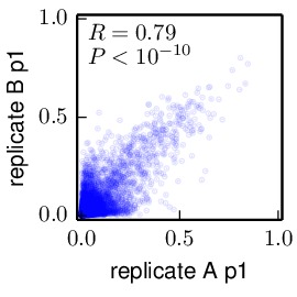
Here is an example of a plot with alpha set to 0.1.