mapmuts_entropycomparison.py
This script is designed to compare the site entropy calculated from the amino-acid preferences between two sets of sites, controlling for solvent accessibility. You might want to use this script to test if one set of sites has a higher site entropy than the other. You are required to know a crystal structure so that you can have computed accessibilities for the residues. The reason is that it is well known that solvent accessibility is correlated with site entropy, so comparing site entropies between sets only makes sense if solvent accessibility is controlled for.
Dependencies
This script requires:
- matplotlib to make the plots.
- rpy2 to run the R statistical package.
- The R statistical package.
Running the script
To run this script, simply create an input file with the format described below. If you name your input file infile.txt, then run the command:
mapmuts_entropycomparison.py infile.txt
Input file
The input file is a text file with a series of key / value pairs. The required keys are indicated below. The values should not include spaces.
Lines beginning with # and empty lines are ignored.
Keys for the input file:
aapreferences : The name of the file giving the site-specific amino-acid preferences \(\pi_{r,a}\). Typically this would be the
*_equilibriumpreferences.txtfile created by mapmuts_inferpreferences.py. These site-specific amino-acid preferences are used to calculate the site entropies.The file has a header, and then for each site r there is a line giving the site entropy \(h_r\) and all of the preferences \(\pi_{r,a}\). It is acceptable for a preference for a stop codon (denoted by a * character) to be either present or absent – but all other 20 amino acids must always be present. Here is an example of a few lines of such a file:
#SITE   WT_AA   SITE_ENTROPY    PI_A    PI_C    PI_D    PI_E    PI_F    PI_G    PI_H    PI_I    PI_K    PI_L    PI_M    PI_N    PI_P    PI_Q    PI_R    PI_S    PI_T    PI_V    PI_W    PI_Y    PI_*
1   M   0.885694    0.000680047 0.00185968  8.48048e-06 0.00128217  0.0289946   0.000654589 0.0212144   0.0205306   0.0021597   0.00056726  0.876551    0.00130602  0.000789781 0.00144568  0.000414457 0.00071164  0.00126055  0.00167084  0.0352283   0.00176486  0.000905383
2   A   1.1671  0.709575    0.00177747  3.79503e-05 0.00298854  0.00390524  0.00131246  0.00379599  0.000913006 0.00121497  0.000535209 0.00276335  0.00140061  0.000694694 0.0032134   0.00464972  0.000463924 0.000908368 0.254241    0.00335749  0.00137437  0.000876985
3   N   3.2593  0.129992    0.000540239 4.2514e-06  0.00171887  0.0212062   0.0006086   0.102743    0.0431489   0.00524637  0.0771062   0.021714    0.0641921   0.00338082  0.0149898   0.0106522   0.13886 0.0247841   0.00607319  0.0500692   0.282389    0.000581555
includestop : an optional argument specifying whether we count stop codons as possible amino acids when computing the site entropies. There may be stop codons as possible amino acids in aapreferences. If there are not stop codons, then the value of includestop is irrelevant. If there are stop codons, the includestop specifies whether these are included as possible amino acids – if True then they are, if False then they are not. Failing to specify includestop is equivalent to setting it to False.
dsspfile is specifies the solvent accessibilities computed from a crystal structure; these are used to compute the relative solvent accessibility (RSA). You can then use the DSSP webserver to calculate the solvent accessibilities. This script is tested against output from the DSSP webserver, but should probably work on output from the standalone too. Then save the DSSP output in a text file, and specify the path to that file as the value for dsspfile. This script does not currently have a robust ability to parse the DSSP output, so you have to do some careful checks. In particular, you must make sure that residue numbers in the PDB file exactly match the residue numbering scheme used for the rest of this analysis (i.e. the same residue numbers found in aapreferences, and that none of the residue numbers contain letter suffixes (such as 24A) as is sometimes the case in PDB files. It is not necessary that all of the residues be present in the PDB. If there are multiple PDB chains, you can specify them using the dsspchain option. DSSP only calculates absolute accessible surface areas (ASAs); the RSAs are computed by normalizing by the maximum ASAs given by Tien et al, 2013.
dsspchain should specify the chain in the PDB file (such as A) that we want to use. If there is only one chain, you can set this option to None.
plotfile is the name of the output plot that is created. It is a PDF, and so should end in the extension
*.pdf.alpha specifies the alpha value (transparency) for the plot. A value of 1.0 means no transparency, and smaller values (such as 0.2 mean more transparency). If you do not include this value, then alpha is set to 1.0 by default.
siterange specifies the range of residues that are included in the analysis. The value should be two numbers giving the first and the last residues to include in the plots. You would use this option if you want to only consider a certain range of residues. If you want to include all of the residues, just set to this to be the string all.
selectedsites is the name of a file that lists the sites that are the selected subset that we are comparing to all other sites. This should be a text file. Lines beginning with # or empty lines are ignored. All other lines should have an integer as their first number, and this is read as the site number. Any other entries on the line are ignored. So in this example file:
# example selectesites file
1
2
# don't include 3
4 # we do include this residue
specifies that we include residues 1, 2, and 4 as selected sites.
linearmodelfile is the name of a created file that holds the results of the linear model analysis as described in Output below. This file is written in text format.
Example input file
Here is an example input file:
# input file for mapmuts_entropycomparison.py
dsspfile ./PDB_structure/1RVX_trimer_renumbered.dssp
dsspchain A
aapreferences combined_amino_acid_preferences.txt
plotfile corr.pdf
linearmodelfile linearmodelresults.txt
alpha 1.0
siterange 2 365
selectedsites Caton_H1_HA_antigenic_sites.txt
Output
The analysis considers all sites that are specified in both aapreferences and in dsspfile and are also in site range.
There are two output. First, the PDF file specified by plotfile is created. All of the non-selected sites are shown in blue circles, and the selected sites are shown in red triangles. An example plot is shown below:
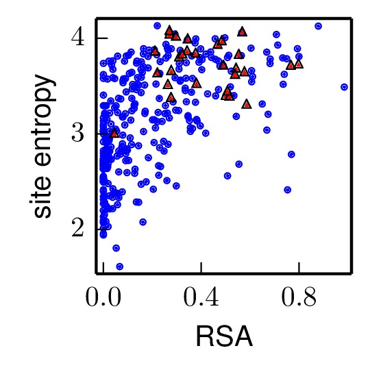
Example of the plotfile plot created by this script.
The second output is the result of an R linear model analysis (R function lm) that looks for the correlations of RSA and presence in selectedsites with site entropy. Essentially, this analysis regresses site entropy against both RSA and the presence in selectedsites (coded as 0 if not in selectedsites, and 1 if in selectedsites). The results of the analysis are written to linearmodelfile. Below is example output. For instance, this example shows that RSA is positively correlated with entropy, and that being a selected site is also positively correlated with diversity:
Residuals:
     Min       1Q   Median       3Q      Max
-1.45241 -0.27611 -0.01408  0.34896  0.96557

Coefficients:
            Estimate Std. Error t value Pr(>|t|)
(Intercept)  2.88267    0.03388  85.090  < 2e-16 ***
RSA          1.29333    0.11903  10.866  < 2e-16 ***
selected     0.29549    0.09276   3.186  0.00158 **
---
Signif. codes:  0 ‘***’ 0.001 ‘**’ 0.01 ‘*’ 0.05 ‘.’ 0.1 ‘ ’ 1

Residual standard error: 0.4563 on 341 degrees of freedom
Multiple R-squared:  0.3238,    Adjusted R-squared:  0.3198
F-statistic: 81.65 on 2 and 341 DF,  p-value: < 2.2e-16